|
|
|
|
Downward continuation |
|
|---|
|
comrecon
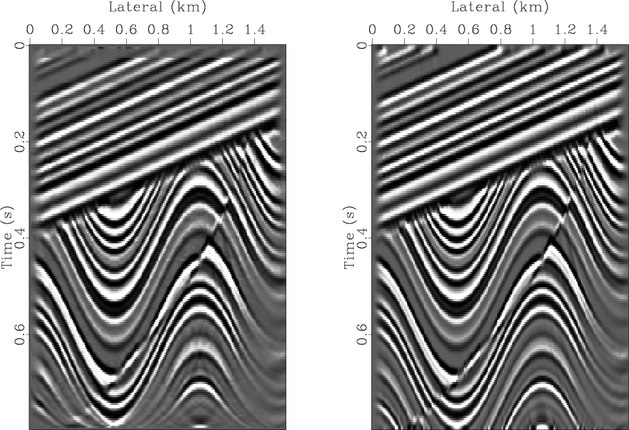
Figure 7. Reconstruction after modeling. Left is by the nearest-neighbor Kirchhoff method. Right is by the phase shift method. |
|
|
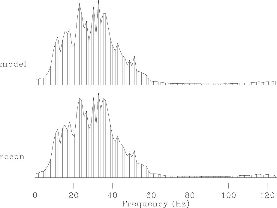
Figure 7.8 shows the temporal spectrum of the original sigmoid model,
along with the spectrum of the reconstruction via phase-shift methods.
We see the spectra are essentially identical
with little growth of high frequencies
as we noticed with the Kirchhoff method
in Figure ![]() .
.
|
phaspec
Figure 8. Top is the temporal spectrum of the model. Bottom is the spectrum of the reconstructed model. |
|
|---|---|
|
|
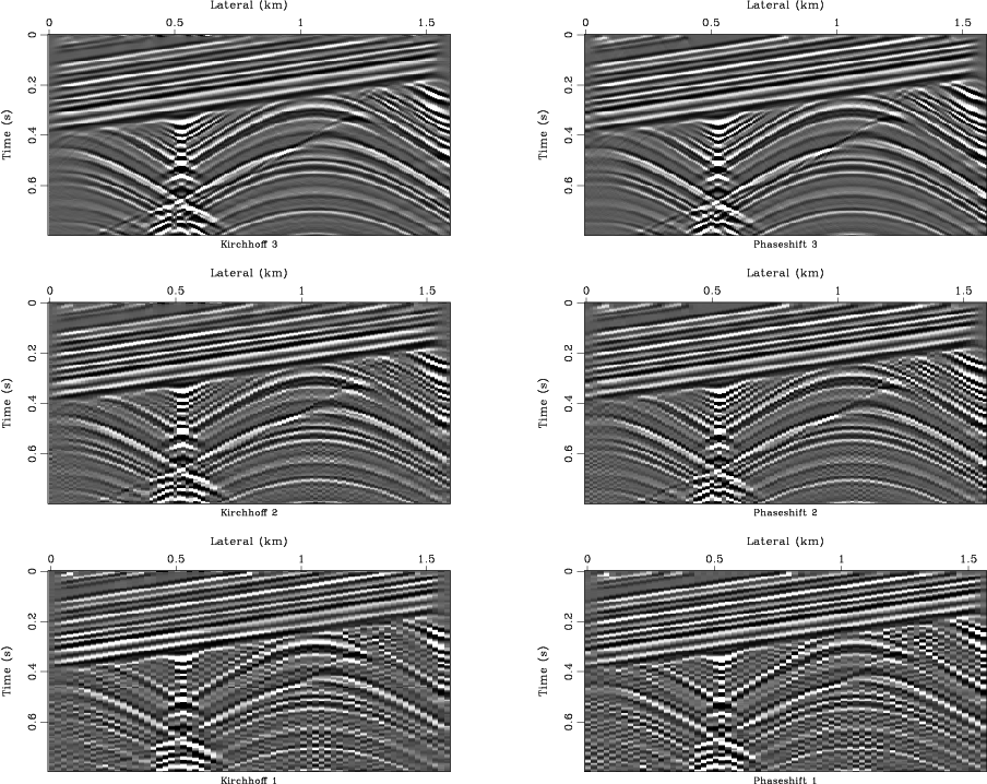
Figure 7.9 shows the effect of coarsening the space axis.
Synthetic data is generated from an increasingly subsampled model.
Again we notice that the phase-shift method of this chapter
produces more plausible results than
the simple Kirchhoff programs of chapter ![]() .
.
|
|---|
|
commod
Figure 9. Modeling with increasing amounts of lateral subsampling. Left is the nearest-neighbor Kirchhoff method. Right is the phase-shift method. Top has 200 channels, middle has 100 channels, and bottom has 50 channels. |
|
|
|
|
|
|
Downward continuation |