|
|
|
|
The Wilson-Burg method of spectral factorization with application to helical filtering |
In the one-dimensional case, one finite-difference representation of
the squared Laplacian is as a centered 5-point filter with
coefficients
![]() . On the same grid, the Laplacian operator
can be approximated to the same order of accuracy with the filter
. On the same grid, the Laplacian operator
can be approximated to the same order of accuracy with the filter
![]() . Combining the two filters in accordance
with equation (6) and performing the spectral
factorization, we can obtain a 3-point minimum-phase filter suitable
for inverse filtering. Figure 4 shows a family of
one-dimensional minimum-phase filters for different values of the
parameter
. Combining the two filters in accordance
with equation (6) and performing the spectral
factorization, we can obtain a 3-point minimum-phase filter suitable
for inverse filtering. Figure 4 shows a family of
one-dimensional minimum-phase filters for different values of the
parameter ![]() . Figure 5 demonstrates the
interpolation results obtained with these filters on a simple
one-dimensional synthetic. As expected, a small tension value
(
. Figure 5 demonstrates the
interpolation results obtained with these filters on a simple
one-dimensional synthetic. As expected, a small tension value
(
![]() ) produces a smooth interpolation, but creates
artificial oscillations in the unconstrained regions around sharp
changes in the gradient. The value of
) produces a smooth interpolation, but creates
artificial oscillations in the unconstrained regions around sharp
changes in the gradient. The value of ![]() leads to linear
interpolation with no extraneous inflections but with discontinuous
derivatives. Intermediate values of
leads to linear
interpolation with no extraneous inflections but with discontinuous
derivatives. Intermediate values of ![]() allow us to achieve a
compromise: a smooth surface with constrained oscillations.
allow us to achieve a
compromise: a smooth surface with constrained oscillations.
|
otens
Figure 4. One-dimensional minimum-phase filters for different values of the tension parameter |
|
|---|---|
|
|
|
|---|
|
int
Figure 5. Interpolating a simple one-dimensional synthetic with recursive filter preconditioning for different values of the tension parameter |
|
|
To design the corresponding filters in two dimensions, we define the finite-difference representation of operator (6) on a 5-by-5 stencil. The filter coefficients are chosen with the help of the Taylor expansion to match the desired spectrum of the operator around the zero spatial frequency. The matching conditions lead to the following set of coefficients for the squared Laplacian:
| -1/60 | 2/5 | 7/30 | 2/5 | -1/60 |
| 2/5 | -14/15 | -44/15 | -14/15 | 2/5 |
| 7/30 | -44/15 | 57/5 | -44/15 | 7/30 |
| 2/5 | -14/15 | -44/15 | -14/15 | 2/5 |
| -1/60 | 2/5 | 7/30 | 2/5 | -1/60 |
| -1 | 24 | 14 | 24 | -1 |
| 24 | -56 | -176 | -56 | 24 |
| 14 | -176 | 684 | -176 | 14 |
| 24 | -56 | -176 | -56 | 24 |
| -1 | 24 | 14 | 24 | -1 |
| -1/360 | 2/45 | 0 | 2/45 | -1/360 |
| 2/45 | -14/45 | -4/5 | -14/45 | 2/45 |
| 0 | -4/5 | 41/10 | -4/5 | 0 |
| 2/45 | -14/45 | -4/5 | -14/45 | 2/45 |
| -1/360 | 2/45 | 0 | 2/45 | -1/360 |
| -1 | 16 | 0 | 16 | -1 |
| 16 | -112 | -288 | -112 | 16 |
| 0 | -288 | 1476 | -288 | 0 |
| 16 | -112 | -288 | -112 | 16 |
| -1 | 16 | 0 | 16 | -1 |
|
|---|
|
specc
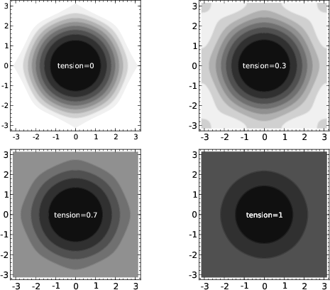
Figure 6. Spectra of the finite-difference splines-in-tension schemes for different values of the tension parameter (contour plots). |
|
|
|
|---|
|
specp
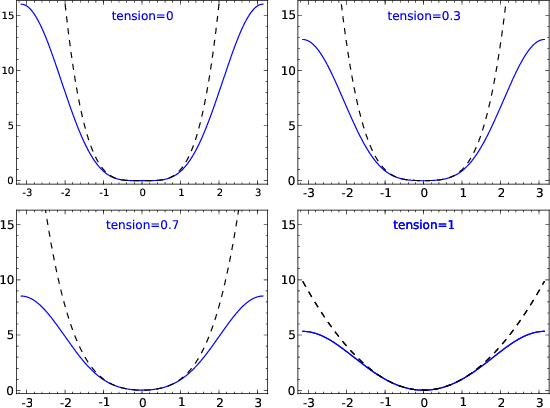
Figure 7. Spectra of the finite-difference splines-in-tension schemes for different values of the tension parameter (cross-section plots). The dashed lines show the exact spectra for continuous operators. |
|
|
Regarding the finite-difference operators as two-dimensional
auto-correlations and applying the Wilson-Burg method of spectral
factorization, we obtain two-dimensional minimum-phase filters
suitable for inverse filtering. The exact filters contain many
coefficients, which rapidly decrease in magnitude at a distance from
the first coefficient. For reasons of efficiency, it is advisable to
restrict the shape of the filter so that it contains only the
significant coefficients. Keeping all the coefficients that are ![]() times smaller in magnitude than the leading coefficient creates a
53-point filter for
times smaller in magnitude than the leading coefficient creates a
53-point filter for ![]() and a 35-point filter for
and a 35-point filter for ![]() ,
with intermediate filter lengths for intermediate values of
,
with intermediate filter lengths for intermediate values of ![]() .
Keeping only the coefficients that are
.
Keeping only the coefficients that are ![]() times smaller that the
leading coefficient, we obtain 25- and 16-point filters for
respectively
times smaller that the
leading coefficient, we obtain 25- and 16-point filters for
respectively ![]() and
and ![]() . The restricted filters do
not factor the autocorrelation exactly but provide an effective
approximation of the exact factors. As outputs of the Wilson-Burg
spectral factorization process, they obey the minimum-phase condition.
. The restricted filters do
not factor the autocorrelation exactly but provide an effective
approximation of the exact factors. As outputs of the Wilson-Burg
spectral factorization process, they obey the minimum-phase condition.
|
|---|
|
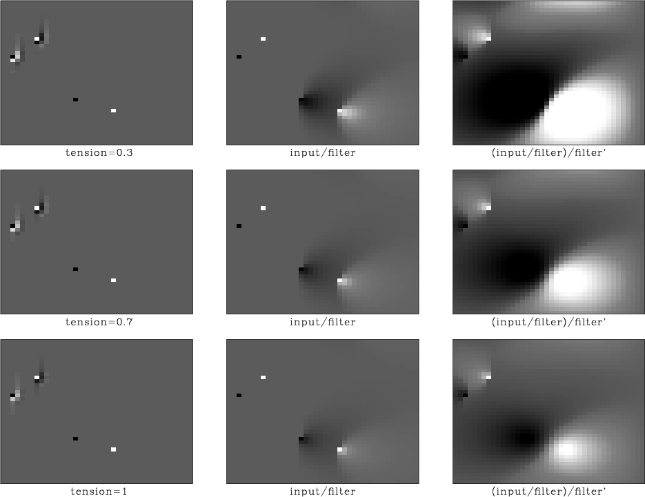
splin
Figure 8. Inverse filtering with the tension filters. The left plots show the inputs composed of filters and spikes. Inverse filtering turns filters into impulses and turns spikes into inverse filter responses (middle plots). Adjoint filtering creates smooth isotropic shapes (right plots). The tension parameter takes on the values 0.3, 0.7, and 1 (from top to bottom). The case of zero tension corresponds to Figure 3. |
|
|
Figure 8 shows the two-dimensional filters for different
values of ![]() and illustrates inverse recursive filtering, which
is the essence of the helix method (Claerbout, 1998). The case of
and illustrates inverse recursive filtering, which
is the essence of the helix method (Claerbout, 1998). The case of
![]() leads to the filter known as helix derivative
(Claerbout, 2002). The filter values are spread mostly in two columns. The
other boundary case (
leads to the filter known as helix derivative
(Claerbout, 2002). The filter values are spread mostly in two columns. The
other boundary case (![]() ) leads to a three-column filter,
which serves as the minimum-phase version of the Laplacian. This
filter is similar to the one shown in Figure 3. As
expected from the theory, the inverse impulse response of this filter
is noticeably smoother and wider than the inverse response of the
helix derivative. Filters corresponding to intermediate values of
) leads to a three-column filter,
which serves as the minimum-phase version of the Laplacian. This
filter is similar to the one shown in Figure 3. As
expected from the theory, the inverse impulse response of this filter
is noticeably smoother and wider than the inverse response of the
helix derivative. Filters corresponding to intermediate values of
![]() exhibit intermediate properties. Theoretically, the inverse
impulse response of the filter corresponds to the Green's function of
equation (6). The theoretical Green's function for the
case of
exhibit intermediate properties. Theoretically, the inverse
impulse response of the filter corresponds to the Green's function of
equation (6). The theoretical Green's function for the
case of ![]() is
is
 . In the case of
In the next subsection, we illustrate an application of helical inverse filtering to a two-dimensional interpolation problem.
|
|
|
|
The Wilson-Burg method of spectral factorization with application to helical filtering |