|
|
|
|
Interferometric imaging condition for wave-equation migration |
Wigner distribution functions (WDF) are bi-linear
representations of multi-dimensional signals defined in phase space,
i.e. they depend simultaneously on position-wavenumber (
![]() ) and
time-frequency (
) and
time-frequency (
![]() ). Wigner (1932) developed these concepts
in the context of quantum physics as probability functions for the
simultaneous description of coordinates and momenta of a given wave
function. WDFs were introduced to signal processing by
Ville (1948) and have since found many applications in signal and
image processing, speech recognition, optics, etc.
). Wigner (1932) developed these concepts
in the context of quantum physics as probability functions for the
simultaneous description of coordinates and momenta of a given wave
function. WDFs were introduced to signal processing by
Ville (1948) and have since found many applications in signal and
image processing, speech recognition, optics, etc.
A variation of WDFs, called pseudo Wigner distribution functions are constructed using small windows localized in space and/or time (Appendix C). Pseudo WDFs are simple transformations with efficient application to multi-dimensional signals. In this paper, we apply the pseudo WDF transformation to multi-dimensional seismic wavefields obtained by reconstruction from recorded seismic data. We use pseudo WDFs for decomposition and filtering of extrapolated space-time signals as a function of their local wavenumber-frequency. In particular, pseudo WDFs can filter reconstructed wavefields to retain their coherent components by removing high-frequency noise associated with random fluctuations in the wavefields due to random fluctuations in the model.
The idea for our method is simple: instead of imaging the reconstructed wavefields directly, we first filter them using pseudo WDFs to attenuate the random phase noise, and then proceed to imaging using a conventional or an extended imaging conditions. Wavefield filtering occurs during the application of the zero-frequency end-member of the pseudo WDF transformation, which reduces the random character of the field. For the rest of the paper, we use the abbreviation WDF to denote this special case of pseudo Wigner distribution functions, and not its general form.
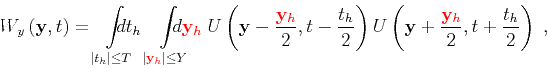
As we described earlier, we can distinguish two options. The first
option is to use wavefield parametrization as a function of data
coordinates
![]() . In this case, we can write the pseudo WDF of the
reconstructed wavefield
. In this case, we can write the pseudo WDF of the
reconstructed wavefield
![]() as
as
For the examples used in this section, we employ ![]() grid points for
the interval
grid points for
the interval ![]() centered around a particular receiver position,
centered around a particular receiver position, ![]() grid points for the interval
grid points for the interval ![]() centered around a
particular image point, and
centered around a
particular image point, and ![]() grid points for the interval
grid points for the interval ![]() centered around a particular time. These parameters are not
necessarily optimal for the transformation, since they characterize
the local WDF windows and depend on the specific implementation of the
pseudo WDF transformation. The main criterion used for selecting the
size of the space-time window for the pseudo WDF transformation is
that of avoiding cross-talk between nearby events,
e.g. reflections. Finding the optimal size of this window is an
important consideration for our method, although its complete
treatment falls outside the scope of the current paper and we leave it
for future research. Preliminary results on optimal window selection
are discussed by Borcea et al. (2006a).
centered around a particular time. These parameters are not
necessarily optimal for the transformation, since they characterize
the local WDF windows and depend on the specific implementation of the
pseudo WDF transformation. The main criterion used for selecting the
size of the space-time window for the pseudo WDF transformation is
that of avoiding cross-talk between nearby events,
e.g. reflections. Finding the optimal size of this window is an
important consideration for our method, although its complete
treatment falls outside the scope of the current paper and we leave it
for future research. Preliminary results on optimal window selection
are discussed by Borcea et al. (2006a).


|
|---|
|
uxx1,wxx1
Figure 4. Reconstructed seismic wavefield as a function of data coordinates (a) and its pseudo Wigner distribution function (b) computed as a function of data coordinates |
|
|


|
|---|
|
uyy1,wyy1
Figure 5. Reconstructed seismic wavefield as a function of image coordinates (a) and its pseudo Wigner distribution function (b) computed as a function of image coordinates |
|
|
Figure 4(b) depicts the results of applying the pseudo WDF
transformation to the reconstructed wavefield in Figure 4(a).
For the case of modeling in the random model and reconstruction in the
background model, the pseudo WDF attenuates the random character of
the wavefield significantly, Figure 4(b). The random character of
the reconstructed wavefield is reduced and the main events cluster
more closely around time ![]() . Similarly, Figure 5(b) depicts
the results of applying the pseudo WDF transformation to the
reconstructed wavefields in Figure 5(a).
For the case of modeling in the random model and reconstruction in the
background model, the pseudo WDF also attenuates the random character
of the wavefield significantly, Figure 5(b). The random character
of the reconstructed wavefields is also reduced and the main events
focus at the correct image location at time
. Similarly, Figure 5(b) depicts
the results of applying the pseudo WDF transformation to the
reconstructed wavefields in Figure 5(a).
For the case of modeling in the random model and reconstruction in the
background model, the pseudo WDF also attenuates the random character
of the wavefield significantly, Figure 5(b). The random character
of the reconstructed wavefields is also reduced and the main events
focus at the correct image location at time ![]() .
.
|
|
|
|
Interferometric imaging condition for wave-equation migration |
![\begin{displaymath}
V_{x} \left ( { \mathbf{x} } , { \mathbf{y} } , { t } \right...
...{ \textcolor{darkgreen}{ {{ t }_h}} }{2} \right)
\right]\;,
\end{displaymath}](img23.png)