Next: The Nyquist frequency
Up: FOURIER TRANSFORM
Previous: FOURIER TRANSFORM
A Fourier sum may be written
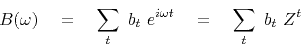 |
(6) |
where the complex value  is related to the real frequency
 by
by  .
This Fourier sum is a way of building
a continuous function of
from discrete signal values
.
This Fourier sum is a way of building
a continuous function of
from discrete signal values  in the time domain.
Here we specify both time and frequency domains by a set of points.
Begin with an example of a signal
that is nonzero at four successive instants,
in the time domain.
Here we specify both time and frequency domains by a set of points.
Begin with an example of a signal
that is nonzero at four successive instants,
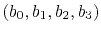 .
The transform is
.
The transform is
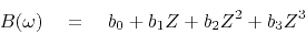 |
(7) |
The evaluation of this polynomial can be organized as a matrix times a vector,
such as
![\begin{displaymath}
\left[ \begin{array}{c}
B_0 \\
B_1 \\
B_2 \\
B_3 \en...
...array}{c}
b_0 \\
b_1 \\
b_2 \\
b_3 \end{array} \right]
\end{displaymath}](img36.png) |
(8) |
Observe that the top row of the matrix evaluates the polynomial at  ,
a point where also
,
a point where also
 .
The second row evaluates
.
The second row evaluates
 ,
where
,
where  is some base frequency.
The third row evaluates the Fourier transform for
is some base frequency.
The third row evaluates the Fourier transform for  ,
and the bottom row for
,
and the bottom row for  .
The matrix could have more than four rows for more frequencies
and more columns for more time points.
I have made the matrix square in order to show you next
how we can find the inverse matrix.
The size of the matrix in (8) is
.
The matrix could have more than four rows for more frequencies
and more columns for more time points.
I have made the matrix square in order to show you next
how we can find the inverse matrix.
The size of the matrix in (8) is  .
If we choose the base frequency and hence
.
If we choose the base frequency and hence  correctly,
the inverse matrix will be
correctly,
the inverse matrix will be
![\begin{displaymath}
\left[ \begin{array}{c}
b_0 \\
b_1 \\
b_2 \\
b_3 \en...
...array}{c}
B_0 \\
B_1 \\
B_2 \\
B_3 \end{array} \right]
\end{displaymath}](img45.png) |
(9) |
Multiplying the matrix of
(9) with that of
(8),
we first see that the diagonals are +1 as desired.
To have the off diagonals vanish,
we need various sums,
such as 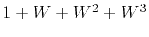 and
and 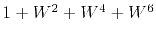 , to vanish.
Every element (
, to vanish.
Every element ( , for example,
or
, for example,
or  ) is a unit vector in the complex plane.
In order for the sums of the unit vectors to vanish,
we must ensure that the vectors pull symmetrically away from the origin.
A uniform distribution of directions meets this requirement.
In other words, should be the
) is a unit vector in the complex plane.
In order for the sums of the unit vectors to vanish,
we must ensure that the vectors pull symmetrically away from the origin.
A uniform distribution of directions meets this requirement.
In other words, should be the  -th root of unity, i.e.,
![\begin{displaymath}
W \quad =\quad
\sqrt[N]{1} \quad =\quad
e^{2\pi i/N}
\end{displaymath}](img51.png) |
(10) |
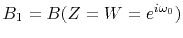
The lowest frequency is zero, corresponding to the top row of
(8).
The next-to-the-lowest frequency we find by setting in
(10) to
 .
So
.
So
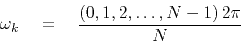
 ; and
for (9) to be inverse to (8),
the frequencies required are
; and
for (9) to be inverse to (8),
the frequencies required are
 |
(11) |
Next: The Nyquist frequency
Up: FOURIER TRANSFORM
Previous: FOURIER TRANSFORM
2013-01-06